
9.1 Solute Transport
The primary mechanisms for solute transport in soil are advection and diffusion. Advection is the transport of solutes due to the bulk flow of water. Diffusion is the net movement of solutes from a region of higher concentration to a region of lower concentration due to the random thermal motion of the solute and water molecules. We will begin our study of solute transport by focusing on these two fundamental mechanisms.
9.1.1 Advection
When water flows through soil with a flux q and a solute concentration C, the resulting advective flux of the solute, Ja, is:
![\[ J_a=q \cdotp C \]](https://open.library.okstate.edu/app/uploads/quicklatex/quicklatex.com-a2aaf611eb97d76b4595127c2068dd00_l3.png "Rendered by QuickLaTeX.com")
(Eq. 9-1)
and has units of mass of solute passing through a unit cross-sectional area of soil per unit time (e.g. g m-2 yr-1). When estimating the distance a solute may travel in a certain amount of time, we need to consider not only the water flux, q, but also the pore water velocity, v. The pore water velocity is the average distance in the direction of the bulk flow which is traveled by an individual water molecule in a unit of time. The pore water velocity depends on the flux and the volumetric water content, θ:
![\[ \nu=\frac{q}{\Theta} \]](https://open.library.okstate.edu/app/uploads/quicklatex/quicklatex.com-959d8aa51df3d64b0b5f95fb4a09c300_l3.png "Rendered by QuickLaTeX.com")
(Eq. 9-2)
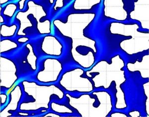
Thus, for a given flux, the pore water velocity is higher when the volumetric water content is lower. If we could measure the water velocities in the soil at the pore scale, we would find a complex pattern of flow paths heading in different directions and at different speeds, as suggested by the simulation results shown in Fig. 9‑1. The average pore water velocity, v, is the net outcome of these innumerable complex flow paths.
Once we know the pore water velocity, we can make a rough estimate of the travel time, t, required for a solute to pass through a layer of soil of specified thickness, L:
![\[ t=\frac{L}{\nu} \]](https://open.library.okstate.edu/app/uploads/quicklatex/quicklatex.com-ebad84f0decbe3a1729fa557bdb16eae_l3.png "Rendered by QuickLaTeX.com")
(Eq. 9-3)
If the soil layer of interest has a uniform water content, we can combine Eqs. 9-3 and 9-2 to get:
![\[ t=\frac{L\Theta}{q} \]](https://open.library.okstate.edu/app/uploads/quicklatex/quicklatex.com-dd249b88763f4c473908d95fb5f1b379_l3.png "Rendered by QuickLaTeX.com")
(Eq. 9-4)
These transport time estimates are only useful for solutes that do not interact in any way with the soil. Adjustments must be made for solutes that interact with the soil, a case we will consider in a later section.
9.1.2 Diffusion
Solute diffusion is the net movement of solutes from a region of higher concentration to a region of lower concentration due to the random thermal motion of the solute and water molecules. Mathematically, this diffusion is governed by Fick’s Law:
![\[ J_d=D\frac{dC}{dZ} \]](https://open.library.okstate.edu/app/uploads/quicklatex/quicklatex.com-cfeab865704ca79b0565fb1c88d600ee_l3.png "Rendered by QuickLaTeX.com")
(Eq. 9-5)
where D is the diffusion coefficient for a particular solute and dC/dz represents the gradient in the solute concentration. The diffusion coefficient for a solute in soil depends on:
- the diffusion coefficient of that solute in pure water,
- the volumetric water content of the soil, and
- the tortuosity of the diffusion paths within the soil pore network.
Solute diffusion in soil is hindered as the soil water content decreases and the tortuosity of the diffusion pathways increases. Thus, diffusion is often a relatively minor contributor to solute transport in soil. However, diffusion can be an important mechanism of transport over small distances, as in the case of nutrient uptake by plant roots.
9.1.3 Hydrodynamic Dispersion
Under the correct circumstances, advection and diffusion interact in a unique way to produce a composite phenomenon called hydrodynamic dispersion. Hydrodynamic dispersion is the process in which the solute appears to be diffusing uniformly upstream and downstream from a plane which is moving downstream at a rate equal to the average pore water velocity. The simulations shown in Fig. 9‑2 show how this dispersion process arises for the special case of flow through a capillary tube.
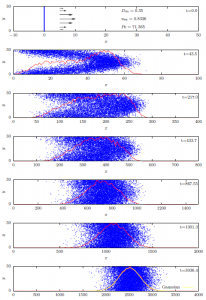
In Poiseuille’s classic work, which we considered in Chapter 4, he showed that flow velocities in a capillary tube have a parabolic distribution with no flow at the tube walls and maximum velocity at the center of the tube. This velocity distribution is indicated by the black arrows on the left hand side of the top panel. When solute is first introduced at a plane in the tube (blue line, top panel) its distribution is impacted by and takes on the shape of that velocity distribution (second panel). The resulting strong concentration gradients in the direction perpendicular to the flow drive strong diffusive transport of solute. This perpendicular diffusive transport has the effect of consolidating and homogenizing the solute distribution over time (panels 3-6), until the distribution becomes a symmetrical, slowly-expanding, normal distribution centered on a plane moving with the average pore water velocity (bottom panel). This rather fascinating and utterly counter-intuitive phenomenon was discovered and described by British physicist Sir Geoffrey Taylor in 1953 [1]. Although soils bear little resemblance to Taylor’s capillary tubes, his representation of hydrodynamic dispersion was soon and widely adopted to describe solute transport in soil [2]. The solute flux associated with hydrodynamic dispersion, Jhd, has been represented as:
![\[ J_h_d=-D_h\frac{dC}{dz} \]](https://open.library.okstate.edu/app/uploads/quicklatex/quicklatex.com-974c8026963fafd3203380304853409c_l3.png "Rendered by QuickLaTeX.com")
(Eq. 9-6)
where Dh is the hydrodynamic dispersion coefficient.
Combining the transport processes considered so far, we obtain an expression for the total solute flux in the soil:
![\[ J_s=J_a+(J_d+J_h_d) \]](https://open.library.okstate.edu/app/uploads/quicklatex/quicklatex.com-4fbd4653b6b6babf8708f3b7e509919f_l3.png "Rendered by QuickLaTeX.com")
(Eq. 9-7)
where the fluxes due to diffusion and hydrodynamic dispersion are grouped together because they cannot be readily distinguished in practice. Inserting the flux equations for each transport mechanism, we obtain:
![\[ J_s=q \cdotp C-D\frac{dC}{dz}-D_h\frac{dC}{dz}=q\cdotp C-D_e\frac{dC}{dz} \]](https://open.library.okstate.edu/app/uploads/quicklatex/quicklatex.com-b4708e4e10dc8b0e4a4c6778bbcbe239_l3.png "Rendered by QuickLaTeX.com")
(Eq. 9-8)
where De is an effective diffusion-dispersion coefficient. This model for the solute transport process has been widely used in soil science, hydrology, and hydrogeology. However, it is only intended to represent the transport of solutes that do not interact with the porous media.
9.1.4 Sorption
Many solutes of interest do, of course, interact with the soil, and one of the most common interactions is the process of sorption. Sorption is a general term for chemical and physical processes by which solutes become attached to soil particles. Examples would include the binding of an organic pesticide like glyphosate by soil organic matter or the attachment of ammonium (NH4+) on a soil’s cation exchange sites. Solutes that undergo sorption are transported less readily than those that do not.
In the simplest cases, we can account for the effects of sorption using a linear adsorption isotherm:
![\[ C_a=K_dC_l \]](https://open.library.okstate.edu/app/uploads/quicklatex/quicklatex.com-181e503071f5521fe60d90ebb3390aa8_l3.png "Rendered by QuickLaTeX.com")
(Eq. 9-9)
where Ca is the adsorbed or absorbed chemical concentration in mass of chemical per mass of dry soil, Kd is the distribution coefficient with units of volume per unit mass, and Cl is the chemical concentration in the solution. When this linear isotherm is valid, we can compute a simple retardation factor, R, to account for the effects of sorption on the solute transport. The retardation factor is given by:
![\[ R=1+\frac{\rho_bK_d}{\Theta} \]](https://open.library.okstate.edu/app/uploads/quicklatex/quicklatex.com-9161ff557839f6a31f26c90fcfc09231_l3.png "Rendered by QuickLaTeX.com")
(Eq. 9-10)
where ρb is the soil bulk density.
We can then introduce this retardation factor directly into Eq. 9-4 to estimate the transport time for a solute subject to sorption:
![\[ t=\frac{R \cdotp L \cdotp \Theta}{q} \]](https://open.library.okstate.edu/app/uploads/quicklatex/quicklatex.com-42b183f1f16d74714a412c3d38aaea92_l3.png "Rendered by QuickLaTeX.com")
(Eq. 9-11)
This equation shows us that the transport time for a solute undergoing sorption is R times greater than the transport time for a solute not undergoing sorption.
9.1.5 Other Processes Impacting Solute Transport
In addition to sorption, a variety of other chemical and biological processes can influence solute transport. Chemical reactions such as oxidation/reduction, dissolution/precipitation, or association/dissociation type reactions can strongly affect solute behavior. Biological processes such as microbial degradation or plant uptake also frequently alter the fate and transport of chemical constituents in the soil. These and diverse other processes can occur simultaneously making accurate prediction of solute transport extremely challenging. Perhaps the single greatest challenge to accurate solute transport prediction arises not from these chemical and biological factors, but rather from instances of severe heterogeneity in the water flow rate, known as preferential flow.
