
2.6 Scale of Primary Soil Particles
When we break down the soil aggregates completely, we are left with the individual soil particles, and the size distribution of these primary particles defines the soil texture. Typically, we classify these particles as either sand, silt, or clay based on their size. In the widely-used classification system of the United States Department of Agriculture, particles < 2.0 and ≥ 0.05 mm are considered sand, particles between < 0.05 mm and ≥ 0.002 mm are considered silt, and particles < 0.002 mm are considered clay. The particle size distribution or soil texture is one of the most significant soil physical properties, and it has a major influence on the chemical, physical, and biological processes that occur in the soil.
To measure the particle size distribution, we typically disperse, or separate, the soil particles in a liquid to create a suspension using either chemical or physical dispersion methods, or both. Sometimes pre-treatment of the sample is necessary to remove binding agents such as soil organic matter. Once the soil particles are completely dispersed and well-mixed in the suspension, the particle size distribution can be determined based on the rate at which particles settle out of the suspension using sedimentation theory. Alternatively, the particle size distribution can be determined using laser diffraction methods, which can also provide information about the particle shape [7].
Sedimentation, or sediment deposition, is the process of particles settling out of suspension, and it is the process most commonly used to determine soil particle sizes and soil texture. You have probably observed that solid particles in a fluid settle at different rates depending on their size and density. In soil science, we often use Stokes’ Law to represent the relationship between a particle’s size, its density, and its settling velocity. For a spherical particle a conceptual diagram of the situation looks like Fig. 2‑12. The symbol, Fg, represents the downward force due to the difference between the weight of the sphere and the buoyancy of the sphere:
![\[ F_g=\frac{4}{3}\pi r^3(\rho_s-\rho_f)g \]](https://open.library.okstate.edu/app/uploads/quicklatex/quicklatex.com-48bbb862936770ec1005fa3db87811e1_l3.png "Rendered by QuickLaTeX.com")
where r is the radius of the particle, ρs is the particle density, ρf is the fluid density, and g is the acceleration due to gravity.
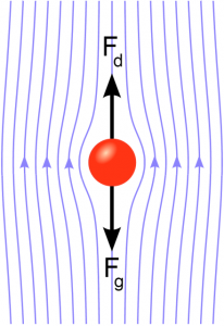
When the falling particle is no longer accelerating, it has reached terminal (or maximum) velocity, and the downward force due to gravity is perfectly balanced by an upward drag force, Fd, due to the particle’s motion through the fluid:
![\[ F_d=6\pi \eta r u \]](https://open.library.okstate.edu/app/uploads/quicklatex/quicklatex.com-96b3d68f986ec5854dc362cfd98d0255_l3.png "Rendered by QuickLaTeX.com")
where h is the dynamic viscosity of the fluid and u is the terminal velocity. The dynamic viscosity is basically a fluid’s resistance to flow and is similar to what might commonly be referred to as the “thickness” of the fluid. Setting Fg = Fd and rearranging, we can solve for the terminal velocity:
![\[ u=\frac{d^2g(\rho_s-\rho_f)}{18\eta} \]](https://open.library.okstate.edu/app/uploads/quicklatex/quicklatex.com-616a599b22ace96fc537b084cab526e9_l3.png "Rendered by QuickLaTeX.com")
(Eq. 2-2)
where d is the particle diameter. Once we know the settling velocity for particles of a given diameter, we can easily calculate the time required for those particles to fall a specified distance through the fluid because velocity is simply distance divided by time. That settling time calculation guides the sampling time used in laboratory methods for determining particle size distribution such as the hydrometer method and the pipette method [8]. For a video explaining and applying Stokes’ Law, click here.
When we use Stokes’ Law to determine the soil particle size distribution, we typically assume that:
- the soil particles are shaped like spheres
- the suspension is dilute enough that the particles do not interact with each other
- the motion of the falling particles is slow enough that it does not generate turbulence
- the particles reach terminal velocity immediately after we stop stirring the suspension
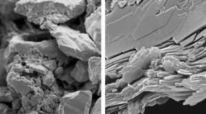
The accuracy of our results then depends on the validity of these assumptions. For example, although sand particles might be roughly approximated as spheres, clay particles resemble something more like thin plates (Fig. 2‑13). Although the shape asumption and others may be violated in standard soil particle size analysis methods, still the application of Stokes’ Law for this purpose has proven to produce reliable and consistent particle size information that is foundational for our physical understanding of soils. If you are curious, you can see the settling behaviour of particles that drastically violate Stokes’ Law demonstrated in this fascinating high speed video (link).
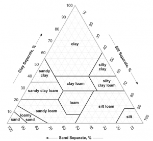
Once we have determined the percentages of sand, silt, and clay in a soil sample, we can identify the soil textural class appropriate for that sample by following the USDA classification scheme or other appropriate national or international schemes. Knowing the sand, silt, and clay percentages, we can use a soil textural triangle to classify a sample (Fig. 2‑14). In textural class names, the last word is the primary classifier and the preceding word or words provide additional descriptive detail. For example, a silty clay is clayey soil with a relatively large amount of silt. In addition to sand, silt, and clay, the words loam and loamy are used to indicate a mix of all three particle size classes.
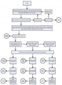
Sometimes we want to estimate soil texture in the field or without the time and expense of the laboratory procedures discussed above. In that case, one can learn, with practice, to estimate the soil textural class accurately by touch and feel, using only a small amount of water. The silent video here and the flow chart below (Fig. 2‑15) describe a widely-used procedure for estimating soil texture by feel according to the USDA soil textural classes [9].
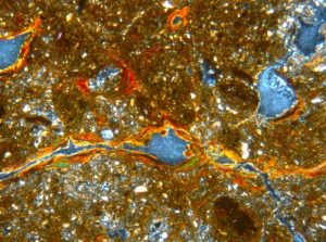
Imagine if you wanted to understand or predict the transport of a pesticide through the soil in Fig. 2‑16 and the pesticide was prone to sorption by the clay. The actual transport behavior might be dominated by water flow through the large pores and by sorption of the pesticide to the clay coatings along those pores, and might be dramatically different from the behavior you would observe if you homogenized the sample and destroyed the micro-scale spatial organization. Researchers have often used disturbed and homogenized soil samples to study soil properties and processes in the laboratory, but in part because of advances in high resolution soil visualization technologies, the strong influence of micro-scale soil organization and the necessity to study the soil intact are becoming increasingly clear.Even when considering soil at the scale of the primary soil particles, we need to recognize that soil is not a homogeneous mixture of particles. Even at this scale where distances are measured in microns, intricate and influential spatial patterns and spatial organization are the rule, not the exception. Consider the beautiful microscopic image below of clay coatings along the pore walls inside a soil from Italy (Fig. 2‑16). Coatings like these typically result from the transport of clay particles by water flowing through the soil pores and deposition of those particles along the pore walls.
